We often use the phrase “the trend is your friend” when analysing noisy data, primarily because it’s a pretty good rule of thumb for the type of polling, economic and demographic data we usually deal with round these parts. Yet sometimes, with certain types of data that exhibit autocorrelated random noise, the “trend”, particularly any local trend witnessed across a relatively short time period, can be extremely deceptive.
To demonstrate, first up we’ll create a really simple time series of data that will become the “reality we are trying to find” for the rest of the post. It will be the “real trend” we will try to find after we swamp it with random noise.
This trend is pretty simple – at observation zero it has a value of zero, at observation 1 it has a value of 0.05, at observation 2 it has a value of 0.1 – each observation the value of this series increases by 0.05. If we look at the first 20 observations of this series, it’s a standard straight line:
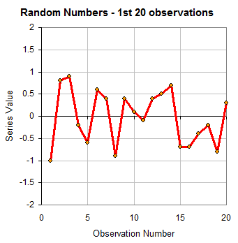
Next up, we need to create some random noise to overlay onto this trend – but we need to make that random noise similar to the sorts of wandering behaviour that regularly infects real world data series. This requires a two stage process, the first part of which is to simply generate some random numbers. For every observation, we will generate a random number between 1 and minus 1 inclusive, to 1 decimal place – so the numbers that will be randomly generated will be out of the set (-1, -0.9, -0.8, -0.7, -0.6, -0.5, -0.4, -0.3, -0.2, -0.1 0, 0.1, 0.2, 0.3, 0.4, 0.5, 0.6, 0.7, 0.8, 0.9, 1)
Our first 20 observations of our random number series look like this:
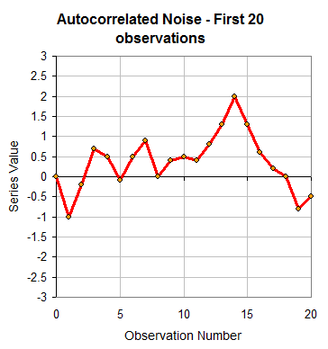
Next, we’ll autocorrelate this series of random numbers for each observation (EDIT: autocorrelation is where the the value of a series at any given point is correlated with, in this instance, it’s most recent value). To start, our zero observation will have a value of zero and our first observation of our autocorrelated series will have the same value as the first observation of our random number series – which in this case is -1.
That’s just required to start the series off. Now, the value of observation 2 will be the 2nd observation of the random number series (0.8) PLUS the previous observation of our autocorrelated series (-1), to give us a value of -0.2. The 3rd observation of our autocorrelated series will be the 3rd observation of our random number series(0.9) plus the 2nd observation of our autocorrelated series (-0.2) …..etc etc. The value of the Nth observation for the autocorrelated series will be the Nth value of the random number series plus the (N-1)th value of our autocorrelated series.
This is what the first 20 values of this now autocorrelated random noise looks like.
It’s worth noting at this stage that the noise involved is much larger than the observation by observation increase in our “real trend” data. Our real trend data increases by 0.05 every period, but the noise can change by as much as 1 or minus 1, a 20 times larger increase than our real trend data, but in either direction.
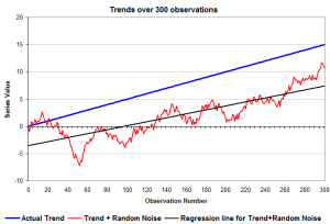
What we do next to get a noisy version of our real trend data is simply to add the autocorrelated random noise series to our real trend series. If we do this for 300 observations, we can compare how our Actual Trend (the real data we are actually trying to find) compares to the Trend + Random Noise (the type of series that we would see in real life)… (click to expand)
What I’ve also added here is a simple linear regression line through that Trend+Random Noise series. What is interesting at this stage is how the noisy series is behaving fairly differently to the Actual Trend series that is its underlying basis.
If you were an economist, or a statistician or some other data scientist and you were given a series of data to analyse, it will often look like the red series above. The problem to be solved is what the real, underlying trend data might actually be. We know what the real trend is – it’s the blue line marked “Actual Trend” – but trying to figure that out without knowing it can be a complicated process, especially when the series has a lot of autocorrelated noise in it.
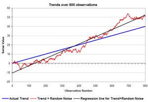
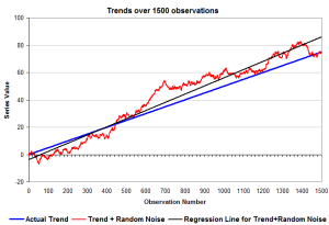
Let’s now look at the first 800 and 1500 observations:
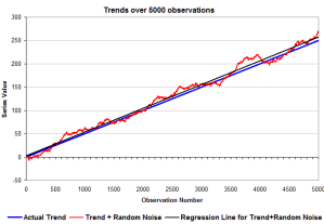
As the number of observations increases, the noisy series slowly starts to converge on to the Actual Trend. If we now move on to the first 5000 observations, it really starts to become apparent:
Over an infinite number of observations, the regression line through the “Trend + Random Noise” series would become identical to the Actual Trend that is our underlying data we would be attempting to find.
What is worth pointing out at this stage, is that even over large numbers of observations, series with autocorrelated random noise (or series where more than one thing is influencing it) can produce local trends that are not representative of the the real Actual Trend underlying the data – trends can be deceptive even after hundreds or thousands of observations depending on the nature of the time series we are looking at.
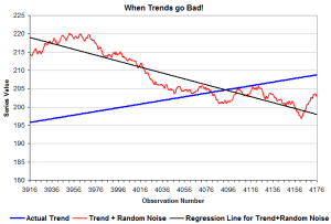
Let’s now take a look at a small subsection of the series and run the numbers again, but where the regression line for Trend+Random Noise is just taken over the sample that is on the chart – it’s 260 observations long.
The local regression would have us believe that there has been a decline in the value of the series over this period, and a statistically significant one at that – even though we know that the Actual Trend has continued to increase at 0.05 units per time period. If this occurred in the real world with some real, important data series – we’d have 3rd rate columnists in the the press banging on about “Teh Decline!!!!!!”, accusing those professionally trained people that would be attempting to point out the “Actual Trend” as being dishonest conspirators.
This brings me back to the problem of people talking about things like “temperature decline since 2001” and the type of arguments used by some in comments in our post about it.
Folks, it’s an exercise in whistling out your arse – you are essentially arguing about random variation so large that it swamps any underlying trend.
Hopefully, from this, you can see why and how that happens, and why and how it is not only futile, but meaningless.
What is important is the larger trends over larger time spans and any structural change that might be measurable in a series, not twaddle about the behaviour of random noise over a short time frame.






Crikey is committed to hosting lively discussions. Help us keep the conversation useful, interesting and welcoming. We aim to publish comments quickly in the interest of promoting robust conversation, but we’re a small team and we deploy filters to protect against legal risk. Occasionally your comment may be held up while we review, but we’re working as fast as we can to keep the conversation rolling.
The Crikey comment section is members-only content. Please subscribe to leave a comment.
The Crikey comment section is members-only content. Please login to leave a comment.